Navigating This Slide Deck
This slide deck uses a two dimensional layout, with multiple vertical stacks of slides arranged left-to-right.
Navigation on desktop computers is straightforward. Simply use Page Up and Page Down (or ← and →) to navigate through all slides sequentially.
On touch devices, you may need to note the graphic in the bottom right to see which additional slides are available and swipe in the appropriate direction: the intended order of slides is top-to-bottom, then left-to-right.
Conducting
Valid Trials
The Critical (and Misunderstood) Roles
of Randomization and Complete Follow-Up
Society for Clinical Trials, May 15, 2016, Montréal, Québec
Presenters:
- Thomas D. Cook, Department of Biostatistics and Medical Informatics,
University of Wisconsin – Madison - Kevin A. Buhr, Department of Biostatistics and Medical Informatics,
University of Wisconsin – Madison - T. Charles Casper, Departments of Pediatrics and Family and Preventive Medicine,
University of Utah School of Medicine
A note to participants: Our workshop will include a number of interactive demonstrations and diagrams that haven’t been reproduced here. Still, we hope that this transcript will be helpful, and we look forward to showing you the “missing data” on Sunday at SCT!
Valid Trials
What is a Valid Trial?
Our definition …
A valid trial is a trial that establishes, up to a predetermined level of statistical certainty, whether an experimental treatment is superior (or non-inferior) to a control treatment.
Importantly, the sole source of uncertainty allowed by this definition is statistical by which we mean non-systematic, random variation.
Therefore, the goals of an investigator conducting a valid trial must be to:
- limit the impact of random variation, in particular by ensuring that the trial has sufficient sample size
- eliminate (to the greatest extent possible), all other sources of uncertainty.
If any systematic sources of uncertainty remain, the validity of the trial is diminished, and whether the trial is salvageable will depend on a subjective assessment of the potential impact of the systematic error.
Given that rescuing an invalid trial requires expert judgment, we propose an alternative statement of the goal of the trial:
to establish a treatment’s effectiveness to the satisfaction of a skeptic who is not prepared to believe the treatment is effective without convincing evidence.

We note that this goal explicitly puts the burden on the investigator/sponsor of the trial to conduct a trial that will be convincing, not just to themselves, but to the broader scientific community.
In our experience, all too often, study sponsors choose to design, conduct and analyze trials in a way that they believe will maximize the chance that they will “win.”
Rather, study sponsors have an ethical obligation to
- patients in the trial
- future patients
- the scientific community
to conduct a trial according to the highest possible scientific standards.
Conventions and Context
Clinical Trials
For the purpose of this workshop, we will consider trials in which we have
- two treatments: control (A) and experimental (B)
- a single primary outcome of interest
- each subject assigned a single treatment
- a statistical test of superiority (except as otherwise noted)
Hypotheses versus Estimation
For a number of reasons, we will also focus on hypothesis testing, rather than estimation.
We will ask …
Is treatment B superior to treatment A?
rather than …
How large is the effect of treatment B relative to treatment A?
In my class I show students a list of mythical creatures:
- Unicorns
- Bigfoot
- Loch Ness Monster
- Yeti (Abominable Snowman)
- β (Treatment Effect)
Why is β a mythical creature?
- It is unclear that there is a coherent definition of “treatment effect.”
- Many of the misconceptions people have regarding trial conduct and analysis stem from an overemphasis on estimation.
- Trials are designed around hypothesis tests with specified power. There is usually no mention of estimation in the sample size calculation.
- It’s difficult to conceive of a universe in which the effect of treatment can be fully captured by a single number.
Inference in Clinical Trials
Inference in Five Easy Steps
Inference in Clinical Trials proceeds according to the following steps …
- Enroll a group of subjects from the target population
- Randomly assign individual subjects to either the experimental treatment or the control treatment
- Ascertain outcomes for each enrolled subject
- Statistically compare the two treatments
… and the final step:
If, to the desired level of statistical certainty, on average the outcomes in the experimental treatment group are superior to those in the control group, then we conclude that the experimental treatment is superior to the control treatment.
This step requires a profound leap of logic!
This is because …
Statistical comparisons are simply computations involving observed data from which we draw conclusions about the distributions of the underlying data.
However, claims regarding the effectiveness of treatment are inherently about causal relationships in the physical universe.
Statistical analysis and causation are independent, unrelated concepts.
It is by the magic of randomization that we are able to make this leap.


Statistics versus Causation
Consider this diagram.
For a given dataset, statistics can assess whether there are associations among these four features.
Now we add arrows.
The arrows represent causal pathways by which treatment with a statin might provide benefit.
Statistics can’t tell us anything about the direction of the causal pathways, or even that they’re causal at all!
Maybe:
- Someone with high LDL has an MI.
- Post MI they’re taken off statins, and subsequently die from the MI.
Unless we know, for example, the temporal relationship (non-statistical!) between these features, we may not be able to rule this out.
Maybe there is some unknown fifth factor that simultaneously changes all four of these and induces the observed association.
Maybe:
- Death reaches backwards in time, causing an MI and elevated LDL.
- The MI and elevated LDL reach backwards in time and cause the subject to not take a statin.
We likely reject this because we believe that causes can only work forward in time, not because of statistics!
Fun fact: There is no statistical evidence showing causes only work forward in time.
In every one of these scenarios (including the “reverse time” scenario), the statistical associations might be exactly the same! We need other, non-statistical, criteria to distinguish between them.
To the extent that we believe this version of the figure, we do so by incorporating non-statistical evidence, both direct and indirect.
For example, we believe, based on RCTs, that Statins lower LDL and risk of MI and Death.
We have statistical associations between LDL and MI/Death, and coupled with biological evidence, conclude that the association is causal.
The Fabled Land of Statistics
Imagine the land on the left side of this figure represents the universe of data and computation, while the right side represents our knowledge of our physical universe.
Every computation that we perform occurs in “Statistics Land” and therefore statistical computation cannot bridge the gap between these worlds. We require another way across.
Our skeptic is acting as the troll preventing anyone from crossing unless their study design and conduct, combined with proper statistical analysis, allow for meaningful inference about how the world works.


Statistics versus Science
Statistical analyses fall into two broad categories …
- Descriptive statistics, where there is no attempt to draw conclusions beyond the sample at hand.
- The mean value of variable X is 53.
- 54% of our sample has Y = 2.
- Statistical inference, where the goal is to gain generalizable knowledge about the distribution of Xs and Ys in the universe from which a sample has been drawn.
- The mean value of X in the population is 53 with 95% CI (42,64).
- The mean of X is larger when Y = 2 than when Y = 1.
Scientific inference is distinct from statistical inference. Scientific inference means describing or drawing conclusions about how the world works.
Broadly speaking, scientific inference falls into two primary categories …
- Correlational or predictive inference, where the goal is to identify characteristics that vary together in the population.
- Older people have higher risk of mortality than younger people.
- People with high HDL (“good” cholesterol) are at lower risk for cardiovascular disease than those with low HDL.
… and …
- Causal inference, where the goal is to infer that X causes Y.
- Statins reduce risk of cardiovascular disease relative to placebo.
We illustrate this distinction by dividing the physical universe on the right into two separate domains.
A statistical hypothesis is a claim regarding a statistical parameter.
For example, given two groups A and B, if β is the difference between the mean response in group A and the mean response in group B, some statistical hypotheses are:
- β=0
- β≠0
- β>0
- 10<β<20
A scientific hypotheses is a claim regarding the true state of nature.
For example, given two treatments, A and B and given a participant population, some scientific hypotheses are:
- Treatments A and B are equally effective
- Treatment A is less effective than treatment B
- Treatment A is more effective than treatment B by 10 units
The scientific goal is to use data and statistics to assess the scientific hypotheses of interest. This requires a link between statistical and scientific hypotheses.
Suppose we construct a confidence interval for β. We would like for there to be a corresponding “confidence interval” for scientific hypotheses as well.
A valid trial is one in which we align our statistical and scientific hypotheses.
We reject:
- H0:β=0
if and only if we reject
- H0:treatments A and B are equally effective
Poll
What allows us to infer WHY two groups are different (causality)?
- Mom
- Randomization
- Assumptions
- Good covariate balance
- Correlation
- The President
Statistics versus Science
Our goal is to convince you that:
Randomization coupled with complete follow-up and an intention-to-treat analysis is the only objective way in which statistical and scientific hypotheses can be aligned.
A Real-World Example
From Ogasa et al. (Psychopharmacology, 2012),
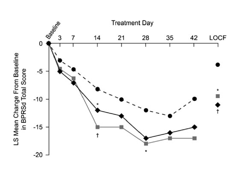
Primary outcome: change from baseline in BPRSd score at 6 weeks.
| Treatment Group | Number Randomized | Number (%) completing |
|---|---|---|
| Lurasidone 40 mg/day | 50 | 16 (32.0%) |
| Lurasidone 120 mg/day | 49 | 20 (40.8%) |
| Placebo | 50 | 15 (30.0%) |
- Primary outcome observed on less than half of randomized subjects.
- Primary analysis uses last-observation-carried-forward (LOCF) for subjects not completing study.
- The plotted trajectories are based on least squares means from an ANCOVA model, a hard-to-understand “black box”.
- Because we don’t observe the 6-week outcome on all randomized subjects, our “skeptic” has no way to know whether the active treatments are really better than placebo or whether the observed differences are due to lack of adherence and follow-up.
Hope-Based Analysis
This analysis might be considered to be based on hope.
We make certain assumptions:
- LOCF reflects the 6-week outcome
- Observations are “missing at random,” so the statistical hypotheses tested using the ANCOVA model align with the scientific hypotheses of interest.
and we hope that they’re correct.
Because our skeptic has no way to verify that these assumptions are correct, he might have good reason to conclude that this is a completely failed trial.
Effect of Missing Data on Alignment of Hypotheses
If we had complete data, our hypotheses would align
With a modest degree of missingness, the extent of misalignment may not be too large.
In this example, the extent of missingness compromises the result of the trial.
Bridges to Causation Land
Observational studies require two steps to assess causal relationships.
The first step uses statistical models to deduce correlations between risk factors and outcomes of interest.
If we can assume that the data at hand are a random sample from the overall population of interest, we can safely cross from Data Land into Correlation Land.
On the other hand, randomization coupled with proper study conduct and analyses is a bridge that gets us directly from Statistics Land to Causation Land.
Convincing Analysis
So, what would our skeptic want to see?
- A simple direct comparison of responses at 6 weeks
- for all randomized subjects
- analyzed according to their assigned treatment groups
- regardless of their adherence to their assigned treatments.
Anything short of this requires our skeptic to trust in some unverifiable assumption made by the investigator/analyst.
A Hypothetical Example
Suppose we conduct a hypothetical trial in COPD. Subjects with COPD will be assigned to
- placebo (treatment “A”), or
- experimental treatment (treatment “B”)
Our outcome will be FEV1% measured 6 months after baseline.
We collect information at baseline:
- age
- smoking status (current, former, never)
- height
- weight
- (baseline) FEV1%
- disease duration
The Purpose of Our Trial
Our scientific conclusions require two steps:
- Statistical inference: “Are the two groups different?”
- Scientific inference: “Is the difference due to an effect of treatment?”
Let’s talk about the role of statistics in this process.
The Role of Statistics
Heterogeneity
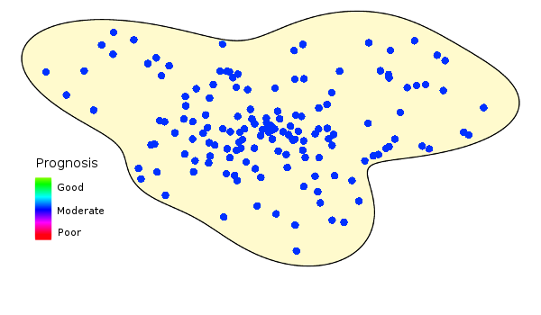
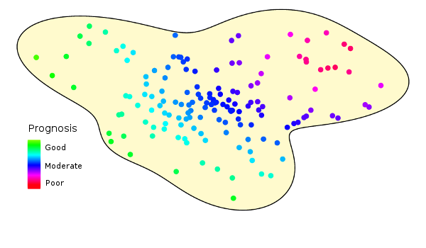
Here’s the hypothetical population we want to study in our trial.
Unfortunately, populations don’t look like this:
Study populations are inherently heterogeneous. This figure illustrates how prognoses vary over a hypothetical population.
Prognosis and Outcomes
Let’s imagine our heterogeneous population distributed along the x-axis of this graph, ordered by severity of the underlying condition (i.e., health status or prognosis).
The y-axis represents the expected response.
Note that the x-axis represents subject status at study start, and is (at least in part) unobservable. The y-axis represents the measured outcome at the study conclusion.
Because populations are heterogeneous, an arbitrarily chosen individual will have different baseline characteristics, different prognosis, and different outcome.
To try to characterize the outcomes across the population, we might take a sample and calculate its mean. This will vary from sample to sample.
The variability of the mean is dependent on the sample size, of course.
However, because the population is heterogeneous, both the magnitude and variability of the sample mean depend on the kinds of subjects we sample.
Comparing Groups
But we’re not interested in describing a typical response. We want to compare groups. Let’s consider two groups defined by some as yet unspecified criteria.
We can imagine two possible outcome curves, one representing group “A”, and the other representing group “B”.
As before, we can take samples from each group and calculate the sample means.
On what basis should we compare them to see if they are different?
Hypothesis Testing
There are two hypotheses of interest:
- The null hypothesis says that the groups are not different, e.g., the true average response is the same in both groups.
- The alternative hypothesis says that the groups are different, e.g., the average in one group is larger than the average in the other.
Before collecting any data, the null hypothesis is assumed to be true and the statistical goal is to show that the null hypothesis is false.
A common approach is to reject the null hypothesis if the difference between the group means is large compared to their standard errors.
We note that were we to sample different kinds of subjects the observed responses differ in several ways, which can affect our hypothesis test.
What if we sample from a more homogeneous, “healthier” subpopulation? The responses in the two groups are larger on average and less dispersed.
Also, because we’ve sampled from a subpopulation that has a smaller average group difference, the observed difference is smaller.
Instead, what if we sample from a more homogeneous, “sicker” subpopulation. The responses in the two groups are now smaller on average but, as above, are less dispersed.
Also, because we’ve sampled from a subpopulation that has a larger average group difference, the observed difference is larger.
Poll
Statistics can tell us WHY two groups are different.
- True
- False
Hypothesis Testing
Note that we haven’t made any claims about the reason the groups are or are not different.
- Statistics can only tell us if groups are or are not different.
- The reason they are different is a causal question and can’t be identified statistically.
In particular, suppose our samples are chosen in a group-dependent way (healthy “A” subjects and sick “B” subjects).
This is confounding — a baseline characteristic that is associated with both treatment and outcome.
The result of the (extreme) confounding in this example is a reversal of the effect, commonly known as “Simpson’s paradox”.
Again, the Purpose of Our Trial
But we do want to show that the reason for a statistical difference is treatment. We want to show that treatment causes a difference in outcomes. So, what do we do?
Causation
Causation
From Hernán and Robins (unpublished):
Zeus is a patient waiting for a heart transplant. On January 1, he receives a new heart.
Five days later, he dies.
Imagine that we can somehow know, perhaps by divine revelation, that had Zeus not received a heart transplant on January 1, he would have been alive five days later.
Equipped with this information most would agree that the transplant caused Zeus’s death. The heart transplant intervention had a causal effect on Zeus’s five-day survival.
Another patient, Hera, also received a heart transplant on January 1. Five days later she was alive.
Imagine we can somehow know that, had Hera not received the heart on January 1, she would still have been alive five days later.
Hence the transplant did not have a causal effect on Hera’s five-day survival. …
In our context, we say that “X causes Y” if Y would have been different if X had been different. Causation is, at it’s heart, about the question:
What would have happened if …
What would have happened if …
Here’s a “typical” human female in our trial.
We imagine that everyone has labels attached to them.
In this case we know that (at baseline) this is a 45 year old female with a BMI of 29 and FEV1% of 82.
The labels marked “A” and “B” are special.
These represent the outcomes that we would observe if this subject were to receive either treatment A or treatment B.
Suppose that we assign this subject to treatment A, conduct the study, and observe the outcome, in this case “79”.
The quantity behind “Door B” remains hidden.
On the other hand, this subject could have been assigned treatment B.
In this case we would have observed a different outcome, “93” and the quantity behind “Door A” remains hidden.
If we were omniscient, we could open both doors, we would know that the “treatment effect” for B relative to A is 93 − 79 = 14.
(Or maybe, 14 ∕ 82 × 100% = 17%, if we define the “treatment effect” to be percent change from baseline.)
Maybe a secondary outcome is vital status. Suppose the person is assigned treatment “A” and they survive.
We don’t know if they would have survived if assigned B.
The subject may also have survived if they had been assigned treatment “B”.
In this case, we wouldn’t know if they would have survived had they been assigned “A”.
Of course, if we were omniscient, we could open both doors, we would know that there is no “treatment effect” on survival for B relative to A.
There is no causal relationship between treatment and survival in this subject.
In our heterogeneous population, if we were omniscient, we would see both outcomes of every subject and could identify the causal effect of treatment for every individual.
In Reality, We Aren’t Omniscient!
The difficulty is that we only get to see what actually happened. We can never know
what would have happened if …
at least not for individual subjects.
Imagining Twins
Suppose for the moment that we aren’t omniscient, but our population is special.
Every individual has a perfect twin.
Perfect twins are more than identical. They are perfectly identical. Not only are all their baseline characteristics, observed and unobserved, exactly the same …
Even their hypothetical outcomes (“what would have happened if …”) match precisely.
With such a population of twins, we could assign one twin to group A (on the left) and the other twin to group B (on the right).
Note that the observed outcome difference between twins (93 − 79 = 14) is the causal effect (in either twin).
And we could do this for everyone in our trial, creating a sample made up of pairs of perfect twins.
By definition, the average causal effect is the average difference in outcome between twins.
Mathematically, this is equal to the difference between average outcomes of the two groups (because the difference of averages is the average of differences).
In a population of twins, this makes a comparison of group means just as good as being omniscient.
In Reality, There Are No Twins!
Well, okay, there are twins (and one of us is married to one), but there are no identical subjects (“perfect twins”).
Nonetheless, we can approximate a population of perfect twins by applying randomization to a twin-less population.
This only works at the population level.
Randomized clinical trials study populations, not individuals. Thinking too much about individuals can lead one astray.
Randomization
Poll
What is the true purpose of randomization?
- to make the groups comparable
- to provide a causal basis for inference
- to confuse trial participants
- to prevent selection bias
- to balance the baseline covariates
- to give statisticians something to do
Usual Rationale for Randomization
The typical rationale for randomization:
“Randomization tends to
Friedman, Furberg, and DeMets
- produce study groups comparable with respect to known and unknown risk factors,
- removes investigator bias in the allocation of participants, and
- guarantees that statistical tests will have valid significance levels.”
This is largely a true statement (although it’s not entirely clear what “comparable groups” means).
However, it makes no explicit reference to causation.
Our skeptic would argue that the three features above are side effects of randomization and are neither necessary nor sufficient to ensure that we can make valid causal claims.
Real Purpose of Randomization
The act of randomization can be thought of as randomly choosing to open either Door A or Door B.
At a population level, this is the same as opening both doors …
… or (again, only at a population level) this is the same as studying a population of perfect twins.
This works because randomization takes random subsamples of the “A” and “B” twins, and random subsamples have the same distribution as the originals.
By the way, using this way of thinking about randomization, it is impossible for the other labels, age, sex, bmi, etc, to have any effect on the difference in outcomes between treatment groups.
That is, we randomly open either Door A or Door B, and the other labels just “come along for the ride.”
Randomization tends to provide approximate balance among baseline characteristics, but this is neither necessary nor sufficient for the validity of our inference.
In particular, chance imbalances do not invalidate our conclusions.
Baseline Covariates
Baseline Covariates
Let’s look at the role of baseline covariates more carefully.
Obviously, if we are ominiscient, we can open both doors at once, and a subject’s baseline covariates are irrelevant to our assessment of causal treatment effect.
Here, the causal effect of treatment B relative to A is 93 − 79 = 14.
If we considered more baseline covariates …
… or fewer …
… or none at all, it would make no difference.
The causal effect of treatment B relative to A is still 93 − 79 = 14.
Randomization — that is, randomly choosing to open Door A or Door B — allows us to open both doors at once, at the population level.
Whether we have data on some baseline covariates …
… many baseline covariates …
… or none at all, randomization acts in the same manner.
Covariates in a Trial
The situation is the same for a clinical trial of heterogeneous patients.
The outcomes may depend on the covariates:
- sicker subjects might have worse outcomes on either treatment
- subjects with certain covariates might have larger causal treatment effect
But if we are omniscient, the baseline covariates are irrelevant to ascertaining the causal effect of treatment in each participant.
Baseline covariates may help improve the efficiency of our inference.
If so, we may need fewer subjects to draw causual conclusions about the underlying population.
But they do not affect the validity of the inference.
If we aren’t omniscient, we can’t open both doors at once, but we can randomize.
This allows us to (randomly) open Door A for half the subjects and Door B for the other half.
Statistical inference we perform on the random doors we open is equivalent, at the population level, to statistical inference performed on all the doors.
It is valid statistical inference on the causal effect of treatment.
Baseline characteristics come along for the ride. They are not relevant to the validity of the inference.
A random imbalance in one or more baseline covariates can’t change this.
That’s fortunate! Otherwise, the validity of clinical trials would depend on the absence of imbalances in covariates we forgot to measure or couldn’t afford to measure or that hadn’t yet been discovered.
The Effect of Baseline Imbalance
The Importance of Balance
Our claims about randomization and baseline imbalance seem to be at odds with conventional wisdom:
“The primary objective of randomisation is to ensure that all other factors that might influence the outcome will be equally represented in the two groups, leaving the treatment under test as the only dissimilarity.” Treasure and MacRae, 1998
“The difficulty [with randomization] arises from the limited degree to which traditional methods can assure comparability of treatment and control groups.” Taves, 1972
“… imbalance between groups in baseline variables that may influence outcome … can bias statistical tests, a property sometimes referred to as chance bias. Observed differences in outcome between groups in a particular trial could by chance be due to characteristics of the patients, not treatments …” Roberts and Torgerson, 1999
Balancing Strategies
This has led some to propose “balancing strategies” as supplements or alternatives to randomization:
“Some protection against chance bias is given by stratified randomisation or minimisation and by adjusting in the statistical analysis for baseline variables.” Roberts and Torgerson, 1999
In Fear of Imbalance
The arguments in favor of balancing strategies seem to …
- take it for granted that covariate balance, at least for “important” covariates, is desirable or even necessary
- make unsubstantiated claims that covariate imbalance biases or invalidates statistical analysis
- make the specific claim that a trial demonstrating a treatment difference in the presence of a baseline covariate imbalance is not credible: the covariate imbalance, rather than the treatment itself, might have caused the observed treatment difference
There’s no doubt that:
In comparison to balancing strategies, randomization causes chance imbalances in baseline covariates.
Or, if you prefer:
In comparison to randomization, balancing strategies cause the elimination of chance imbalances.
But this isn’t the question of interest.
The question of interest is:
In comparison to balancing strategies, does randomization cause biased or invalid statistical analysis?Specifically, does randomization cause detection of spurious treatment differences that would not have been observed if only we had employed a balancing strategy?
Note that this is a causal question, and we can evaluate it in our causal framework.
Minimization
The minimization scheme for treatment allocation …
- was introduced by Taves in 1972.
- was his response to a clinical trial where a promising treatment did not demonstrate a significant effect which he attributed to an unfavorable chance imbalance in key covariates (i.e., where randomization, through a chance imbalance, caused the trial to fail to show the effect of treatment).
- is a (nearly) deterministic algorithm that allocates each patient in the manner that minimizes the imbalance between groups in a set of one or more prespecified baseline covariates.
Consider a simple example based on sex (M/F) and smoking status (S/NS). The first patient is randomized. Subsequent patients are assigned to the treatment that minimizes imbalance or randomized in case of tie.
| Imbalance | |||||||
|---|---|---|---|---|---|---|---|
| No. | Patient | M | F | S | NS | Total | Trt |
| 1 | Male, non-smoker | +1 | 0 | 0 | +1 | 2 | A |
| −1 | 0 | 0 | −1 | 2 | B | ||
| 2 | Female, non-smoker | +1 | +1 | 0 | +2 | 4 | A |
| +1 | −1 | 0 | 0 | 2 | B | ||
| 3 | Female, non-smoker | +1 | 0 | 0 | +1 | 2 | A |
| +1 | −2 | 0 | −1 | 4 | B | ||
| 4 | Female, smoker | +1 | +1 | +1 | +1 | 4 | A |
| +1 | −1 | −1 | +1 | 4 | B | ||
| 5 | Female, smoker | +1 | 0 | 0 | +1 | 2 | A |
| +1 | −2 | −2 | +1 | 6 | B | ||
| Legend: Randomized and Minimized | |||||||
Causal Effect of Minimization
Let’s determine the causal effect of using minimization instead of randomization to allocate treatment.
Let’s start by considering the effect on the number of “spurious results”.
A spurious result is a trial where we detect a statistically significant treatment difference that is not due to treatment.
To us, this only makes sense in a case where the treatment is ineffective.
Some people might argue that, even if the treatment is effective, a trial result might still be spurious if a finding of effectiveness is because of a baseline covariate imbalance instead of because of the treatment.
This strikes us as pretty stupid meaningless, so we’ll stick with trials where the treatment has no effect.
Consider a comparison of placebo (Door A) with a completely ineffective treatment (Door B). Because the treatment is totally ineffective, the outcomes are the same.
Let’s imagine a clinical trial of this ineffective treatment.
Each subject has the same outcome behind Door A and Door B.
Because we’re omniscient, we can figure out what would have happened if we randomized subjects …
Here, the treatment group difference was 6.4 (in favor of B), p = 0.30.
… and what would have happened if we used minimization.
Here, the treatment group difference was 4.4 (in favor of A), p = 0.48.
This allows us to directly ascertain the causal effect of minimization versus randomization on trial results.
For this particular trial, the treatment allocation method had no causal effect on the spuriousness of the results.
Simulation with Real Data
Of course, that’s only one particular trial. To evaluate the causal effect of minimization in general, we’ll want to look at many trials where we can take an omniscient view.
We can do this through simulation.
To make our simulation as realistic as possible, we’ll use real data.
But we aren’t actually omniscient, so how can we be omniscient while using real data?
Suppose we had real data on COPD patients from a large clinical trial. We’d have their baseline covariates available.
For subjects in the placebo arm, we’d also have their placebo (Door A) outcomes.
If we wanted to use this real data to simulate a completely ineffective treatment (Door B) …
… we’d just copy the outcome from Door A to Door B. That’s the definition of a completely ineffective treatment.
We don’t have data on a large COPD trial.
But we do have data on a randomized clinical trial of 15,000 patients (7500 per treatment arm) of a CETP inhibitor, a drug that raises HDL-C (the “good” cholesterol).
We have:
- real baseline characteristics
- actual Month 3 HDL-C outcomes
We’ll use the baseline characteristics and Month 3 HDL-C of the 7500 placebo patients as our “population” of eligible subjects.
We’ll simulate small trials of a completely ineffective treatment compared to placebo by sampling from this population.
And we’ll study the causal effect of randomization versus minimization in each simulated trial.
A Simulated Trial
If we simulate a single small trial (n=40, 20 per group), we can see the causal effect of minimization compared to randomization on improved covariate balance.

We can also see the causal effect of minimization compared to randomization on the spuriousness of the trial results.
| Mean A | Mean B | Diff | P-value | Spurious? | |
|---|---|---|---|---|---|
| Randomization | 49.8 | 43.3 | −6.5 | 0.11 | No |
| Minimization | 46.3 | 46.9 | +0.3 | 0.88 | No |
Assuming α = 0.05, there was no causal effect on spuriousness for this particular trial, though it does look as if minimization is improving the “accuracy” of the estimate.
Is this typical?
More Simulated Trials
Let’s simulate 100,000 trials and determine, for each one, the causal effect of allocation strategy on spuriousness:
| Minimization | ||
|---|---|---|
| Randomization | Not Spurious | Spurious |
| Not spurious | 91,333 | 3806 |
| Spurious | 4657 | 204 |
In the vast majority of cases (91.5%), there is no causal effect of minimization versus randomization on the spuriousness of the trial.
When balance advocates claim that minimization improves validity of trials, it pays to remember that their “treatment” for invalid trials is completely ineffective 91.5% of the time.
Yes, Randomization Causes Invalid Trials
In about 4.7% of cases, a trial would produce a spurious result if randomization were used, but would not produce a spurious result if minimization were used.
In these case, there is a causal effect of treatment allocation: randomization causes the trial to produce a spurious result, and minimization causes the removal of the spurious result.
These are the trials the balance advocates warned us about! Let’s look at one (chosen at random).
For this trial, here is the causal effect of randomization on trial results:
| Mean A | Mean B | Diff | P-value | Spurious? | |
|---|---|---|---|---|---|
| Randomization | 50.6 | 43.6 | −7.0 | 0.03 | Yes |
| Minimization | 47.8 | 46.4 | −1.4 | 0.65 | No |
It looks like randomization caused the spurious result by slightly increasing the mean in group A and decreasing the mean in group B.
Here’s is the dramatic baseline covariate imbalance that randomization caused and minimization fixed.

Also, Minimization Causes Invalid Trials
Compared to the 4657 cases where randomization causes spurious results, there are “only” 3806 cases where minimization causes spurious results.
(This difference is real, and we’ll explain it in a moment.)
What does it look like when your trial is one of those 3806? Let’s look at such a case chosen at random.
For this trial, here is the causal effect of minimization on trial results:
| Mean A | Mean B | Diff | P-value | Spurious? | |
|---|---|---|---|---|---|
| Randomization | 49.1 | 52.3 | +3.2 | 0.45 | No |
| Minimization | 46.1 | 55.3 | +9.2 | 0.02 | Yes |
Minimization caused the difference to be vastly overstated. How did we go so wrong?
Obviously, minimization caused this invalid result by eliminating crucial imbalances in covariates.

A more serious way of looking at it: even in trials of completely ineffective treatments, balance in covariates does not ensure balance in outcomes.
Just because minimization causes covariate balance, that does not mean it will cause outcome balance.
In fact, in the course of balancing covariates, it may — literally — cause outcome imbalance!
Missed Opportunities
To be fair, we should look at the other side of the coin.
Let’s consider trials of an effective treatment that failed to find a significant difference.
We’ll call these missed opportunities.
Note that a missed opportunity was what inspired Taves to develop minimization in the firist place.
Of course, if the trial lacks power to detect a clinically significant difference, or if the actual treatment effect is too small, the trial may fail.
We will consider adequately powered trials (at least 90% power) for a highly effective treatment.
Once again, we want to simulate a large number of trials as if we were omniscient, but we’d like to do this with real data.
How do we proceed?
We’ll use the baseline characteristics and actual Month 3 HDL-C of the 7500 active treatment patients as our "population" of eligible subjects.
To simulate being omniscient, we’ll use the baseline HDL-C of these subjects as the outcome if they had received treatment A.
Note that this isn’t perfect. If this was the real causal effect of treatment in treated patients, we wouldn’t need control groups. We’d just compare pre- and post-baseline results.
We hope that it’s close enough for a realistic simulation.
A Simulated Trial
Again, let’s simulate a single small trial of n=40 (20 per group) to see the causal effect of minimization compared to randomization on improved covariate balance.
Here’s an example where minimization did a great job fixing a big age imbalance (mean 55 vs. 63 years) in this 40-person trial, one that could have caused a missed opportunity.

… except it didn’t cause anything of the kind. This trial was going to be successful, regardless of allocation strategy.
| Mean A | Mean B | Diff | P-value | Missed Opp.? | |
|---|---|---|---|---|---|
| Randomization | 48.2 | 67.0 | +18.8 | 0.005 | No |
| Minimization | 42.5 | 73.1 | +30.6 | 0.003 | No |
Again, there was no causal effect of minimization versus randomization on missed opportunities for this trial.
More Simulated Trials
Let’s simulate 100,000 trials and determine, for each one, the causal effect of allocation strategy on missed opportunities:
| Minimization | ||
|---|---|---|
| Randomization | Miss | Hit |
| Miss | 16 | 445 |
| Hit | 352 | 99,187 |
As before, in the vast majority of cases (99.2%), there is no causal effect of minimization versus randomization on missed opportunities in detecting a successful treatment.
But maybe the trial that inspired Taves’ came from that pesky 0.8%. (To be fair, this fraction would be slightly larger if the trial had been less well powered.)
Yes, Randomization Causes Missed Opportunities
Again, there’s no escaping the fact that, that, in about 0.4% of our simulations, randomization caused a missed opportunity.
That is, the trial would have been successful in detecting a treatment effect if we had used minimization but would have failed if we had used randomization.
Let’s look at one (chosen at random).
For this trial, here is the causal effect of randomization on trial results:
| Mean A | Mean B | Diff | P-value | Missed Opp.? | |
|---|---|---|---|---|---|
| Randomization | 49.3 | 57.6 | +8.3 | 0.07 | Yes |
| Minimization | 46.4 | 65.5 | +19.1 | <0.001 | No |
Here’s the baseline imbalance that minimization fixed to rescue this trial.

Also, Minimization Causes Missed Opportunities
Compared to the 445 cases where randomization caused a missed opportunity, there were 352 cases where minimization caused a missed opportunity.
(This difference — that minimization caused 0.1% fewer missed opportunities than it prevented — is real. We’ll explain it in a minute, for those who are worried that after discovering 999 highly effective treatments, they might have missed one.)
Let’s look at one of these 352 cases at random.
For this trial, here is the causal effect of minimization on trial results:
| Mean A | Mean B | Diff | P-value | Missed Opp.? | |
|---|---|---|---|---|---|
| Randomization | 50.9 | 75.7 | +24.8 | 0.002 | No |
| Minimization | 55.7 | 67.7 | +12.0 | 0.07 | Yes |
Minimization did another great job balancing covariates. Too bad it wrecked this trial.

The Actual Benefit of Minimization
If you’re like us, you aren’t too impressed that minimization prevented only 0.8% more spurious results than it caused …
| Minimization | ||
|---|---|---|
| Randomization | Not Spurious | Spurious |
| Not spurious | 91,333 | 3806 |
| Spurious | 4657 | 204 |
… and prevented only 0.1% more missed opportunities than it caused …
| Minimization | ||
|---|---|---|
| Randomization | Miss | Hit |
| Miss | 16 | 445 |
| Hit | 352 | 99,187 |
… while having absolutely no effect (useful or otherwise) in 91.5% of trials of ineffective treatments and 99.2% of trials of highly effective treatments.
Still, the fact remains that, in our simulation, the causal effect of minimization was to:
- reduce Type 1 error from about 0.05 to 0.04
- reduce Type 2 error from about 0.005 to 0.004
So it is clearly superior to randomization, right?
Inefficiently Improving Efficiency
What’s really going on?
Minimization is making use of baseline covariate information.
As mentioned before, this can improve efficiency.
Normally, when we use statistical techniques to improve efficiency:
- we increase our power (i.e., decrease our Type 2 error)
- while maintaining the same level of Type 1 error (equal to our choice of nominal α=0.05)
Because minimization is a relatively inefficient way of incorporating baseline covariate information to improve efficiency:
- we increase our power (i.e., decrease our Type 2 error)
- while also decreasing our Type 1 error below our desired level of α=0.05, allowing our tests to become too conservative
To realize the full efficiency gain of using baseline covariate information, we would want to maintain our preselected level of Type 1 error and increase our power even more!
Efficiently Improving Efficiency
In most cases, the best way of incorporating baseline information is to incorporate it into the analysis, not the treatment allocation strategy. This is superior because:
- it can make full use of the information to increase power while maintaining the same type 1 error
- it’s flexible, allowing us to incorporate covariate information we didn’t prespecify
- in large trials, it provides better implicit matching (through modelling) than balancing strategies for large numbers of covariates and/or complex covariate interaction effects
But, I have a confession to make.
In this particular simulation, minimization does a pretty good job of making use of available baseline covariate information.
Because we are considering …
- small trials (n=40)
- where a relatively small subgroup (females, 22%)
- exhibits a big systematic difference in outcome (17% higher than males)
… modelling can’t take full advantage of baseline covariate information in those randomized trials where there are too few females in one group or the other (e.g., where all the females are in group A).
So, minimization leads to a slight efficiency gain. (The gain is about half the gain realized by increasing the sample size from n=40 to n=42.)
However, please note:
- This is not, as balance advocates claim, because the resulting baseline imbalance invalidates the trial (even when all the females end up in group A).
- This is because there are too few females in one group to serve as a proper comparison group for the females in the other group.
- In these cases, the modelling analysis can’t do any better than an analysis that ignores baseline covariates, so opportunities get missed.
Randomization and Baseline Covariates
We’ve established that randomization ensures the validity of the trial, in spite of any random covariate imbalances.
However, there are a few remaining issues.
Some Unspoken Assumptions
We’ve made two key assumptions so far:
- Outcomes are available on all subjects.
- All subjects fully adhere to their treatment and realize the full causal effect on their outcomes.
Missing Data
Poll
If our trial will have missing data, the only effect will be a loss of power. So we just need to enroll more subjects to compensate for the missing data.
- True
- False
The Effect of Missing Data
Unfortunately, virtually all trials have some degree of missing data.
What impact will missing data have on our hypothetical trial?
The assumption is frequently made that observations are missing at random (we’re using this term informally and won’t define it).
If this assumption is correct, the only consequence of missing data is that we have a smaller sample size and, therefore, lower power and precision. Otherwise, the analysis of the available data will give the same results as if there were no missing data.
Sometimes, it’s acknowledged that observations are not missing at random, but the assumption is made that the missingness is not influenced by treatment. (Again, we won’t define exactly what we mean here.)
If this assumption is correct, it can change the results of the analysis, but at least the analysis still has a causal interpretation.
The problem is that, by their very nature, missing data are unobserved and it is impossible to know whether they are actually missing at random.
Non-random, treatment-dependent missingness can easily subvert the benefits of randomization.
Straightforward analysis of such data no longer has a causal interpretation.
Missing Twins
As before, let’s imagine we sample from a population of perfect twins.
Now suppose there are some pairs of twins with a missing outcome.
If we include only complete pairs, we will still have a valid causal analysis.
Having missing pairs in a population of twins is analogous to “missingness is not influenced by treatment” in a randomized, twin-less population.
This is because, even if missingness depends on the attributes of an individual, if twins always go missing in pairs, then treatment (the only difference between twins) is not influencing missingness.
Partly Missing Pairs
But why would data on twins only go missing in pairs? We have to assume that, in some pairs, one twin has complete outcome data, but the other does not.
Again, if we include only complete pairs in our analysis, we will still have a valid causal analysis
However, this requires that we are able to identify “twins”, specifically the twin with complete data that corresponds to the one with missing data, so the former can be removed from the analysis.
If we really were studying a population of perfect twins, this would be easy.
But we are using randomization to approximate a population of twins. If an individual in group A has missing data, there is no perfect twin in group B to remove!
Unmatched Twins
If we proceed to compare everyone in groups A and B anyway, we include in our analysis the differences between twins in the complete pairs (which is a causal effect), plus some extra twins in group A that don’t have a match, and some extra twins in group B that don’t have a match.
We have no reason to believe that the unmatched group A twins are comparable to the unmatched group B twins. We might hope that their differences will “cancel out” to give a causal effect, but this requires untestable assumptions.
Missingness in Our Trial
If the data are missing at random, there is no effect on the causal analysis.
If the data are not missing at random but missingness isn’t influenced by treatment, the analysis changes, but we are still making a causal comparison.
If neither assumption holds, as we’d expect in most real-world trials, then all bets are off.
Even under the scentific null hypothesis (where there is no causal effect of treatment by definition), missingness can create a statistically significant difference.
Note that the statistics is working fine: there is a difference between these groups.
But the randomization has been subverted. The difference can’t be a causal effect of treatment.
Effect of Missingness on Type 1 Error Rates
A Missing Data Example
| Dead | Alive | Missing | Total | |
| A | 38 | 51 | 10 | 100 |
| B | 21 | 70 | 9 | 100 |
To explore the impact of missingness on type 1 error rates, consider this 2×2 table.
Overall, vital status is missing for about 10% of subjects.
Using the complete data, the Pearson chi-square Z statistic is 2.80, p = 0.0051, favoring group B.
What is the impact of the missing data? For this particular table, the answer requires sensitivity analysis, which we’ll discuss later.
For now, let’s just consider the impact of missing data more generally.


Rates of Missingness
Assume for simplicity that the rates of missingness are the same in the two groups, and let’s consider two probabilities:
QA=Pr(dead|missing, group A)QB=Pr(dead|missing, group B)
If these two probabilities are equal, on average there is no net effect of missingness on the overall type 1 error rate.
Now consider the effect of a difference between these probabilities. Suppose that we let QA=20 and consider the effect of the difference QB−QA on type 1 error rate.
The Skeptical Zone
Imagine that there are two plausible zones for QB−QA, an “optimistic” zone, where the difference isn’t too large, and a more “skeptical” zone, where larger differences are considered plausible.
Maybe our skeptic lives in the “skeptical” zone.
Now suppose that the null hypothesis is true so that the true failure rate is the same in both groups and is equal to 30%, and that we have 5% missingness.
Here we have a total sample size of 200. This corresponds to a study that would be powered for a risk ratio of 0.39, or a reduction to 11.7% failure rate in group B.
The actual type 1 error rate increases slightly as QB−QA increases, but is still quite close to 5% in the “skeptical” zone.
If we increase the sample size to 400, we would have power for a risk ratio of 0.55, or a reduction to 16.5% failure rate in group B.
The actual type 1 error rate increases a bit more as QB−QA increases, but is still quite close to 5% in the “skeptical” zone.
Big Samples
If we increase the sample size to 1000, we would have power for a risk ratio of 0.7, or a reduction to 21% failure rate in group B.
The actual type 1 error rate can be significantly above 5%, and rises to as much as 8% in the “skeptical” zone.
For a sample size of 2000, we would have power for a risk ratio of 0.79, or a reduction to 20% failure rate in group B.
The actual type 1 error rate can rise to as much as about 12% in the “skeptical” zone.
For a sample size of 4000, we would have power for a risk ratio of 0.85, or a reduction to 25.5% failure rate in group B. It may be unlikely that a study would be powered for a RR as close to one as this.
Still, the actual type 1 error rate can rise to 18% in the “skeptical” zone.
For a sample size of 10000, we would have power for a risk ratio of 0.9, or a reduction to 27% failure rate in group B. We’re unlikely to see a trial this large in practice.
The actual type 1 error rate rises to about 40% in the “skeptical” zone.
For a sample size of 20000, we would have power for a risk ratio of 0.93, or a reduction to 27.9% failure rate in group B.
The actual type 1 error rate rises to nearly 70% in the “skeptical” zone.
Here are all the previous sample sizes on a single figure.
More Missing Data
Now consider the same set of sample sizes, but with a 10% missingness rate.
The type 1 error rate rises to about 7% in the skeptical zone for n = 200, about 10% for n = 400, and is at least 20% for the remaining sample sizes.
If the missingness rate increases to 15%, the type 1 error rate rises to about 12% in the skeptical zone for n = 200, about 18% for n = 400, and is at least 40% for the remaining sample sizes.
Finally, for a missingness rate of 20%, the type 1 error rate rises to about 18% in the skeptical zone for n = 200, about 33% for n = 400, and is over 65% for the remaining sample sizes.
As noted, the two largest sample sizes are unlikely to be seen in practice, but between 400 and 4000 are plausible sample sizes, and the type 1 error rates may be seriously inflated, even within the “optimistic” zone.
Missing Data for Big Trials
In trials powered for relatively small reductions in risk (RR ≥ 0.8), a missingness rate of as little as 5% can dramatically increase the type 1 error rates under skeptical (yet plausible!) assumptions.
When missingness rates exceed 10% in studies powered for all but the largest reductions (RR ≥ 0.5), type 1 error rates can be dramatically affected.
If missingness rates exceed 15%, nearly all reasonably sized trials can be seriously compromised.
Handling
Missing Data
Missing Data Methods
Common approaches when data are missing:
- Complete-case analysis
- Imputation
- Principal Stratification
- Joint modeling of outcome and missing indicator
- Inverse probability methods
Poll
If we have missing data, which of the following methods will allow for a "hope-free", causal interpretation of the results?
- Complete-case analysis
- Imputation
- Principal stratification
- Joint modeling
- Inverse probability weighting
- All of the above
- None of the above
Complete-case Analysis
In complete-case analysis, we just analyze all subjects with complete data.
We’ve already seen that this is not a valid causal analysis.
Imputation
Imputation means “filling in” the missing values in some principled way. Of course, this can only done be making untestable assumptions.
We have to make assumptions and hope they’re correct.
Imputation Methods
- Last observation carried forward (LOCF)
- Single imputation
- Multiple imputation
Last Observation Carried Forward
Use the last value that was observed before data collection ceased.
- One of the most popular approaches (unfortunately)
- Some have argued it provides a conservative estimate of treatment effect
Assumes that either:
- The missing outcome is EQUAL to the last observed value (which is unverifiable and unrealistic)
- The outcome of interest is actually “your final value before you drop out” (which is scientifically absurd)
If we took an omniscient look at a particular subject’s Month 3 data, we might see the subject get worse under treatment A but maintain her baseline value under treatment B.
The causal effect of treatment of B relative to A at Month 3 is 82 − 69 = 13.
If we forced this subject to provide us with Month 6 data, an omniscient look at her outcomes might show a treatment effect at Month 6 of 93 − 79 = 14.
Note that the subject shows improvement since Month 3 under either treatment, though the causal treatment difference at each time point is similar (13 vs. 14).
Maybe the subject had a bad cold around Month 3 but is now recovered.
Suppose that, if we hadn’t forced our subject to show up for Month 6, she would have discontinued the trial at Month 3 under treatment A (when her FEV₁% dropped to 69) but would have kept going under treatment B.
Here, the causal effect of treatment on outcome and timepoint is shown.
LOCF ignores the timepoint difference and estimates a treatment effect at Month 6 of 93 - 69 = 24, almost double the true causal effect.
But remember, LOCF is supposedly "conservative"!
We aren’t omniscient, but we can randomize. This lets us open both doors at once at a population level.
If we use LOCF, this subject’s contribution, on a population level, will be the misleading effect size of 93 - 69 = 24.
- Contrary to some claims, LOCF is not guaranteed to be conservative.
- For example, even when the “treatment effect” is conservatively estimated, the variability can be underestimated.
- It is also very easy to construct examples where the LOCF estimate is anti-conservative.
- LOCF has no causal basis.
Single Imputation
Single imputation involves filling in the missing value. We might do this using:
- a simple mean
- a regression or other modelling approach
(Note that LOCF is a type of single imputation.)
Single imputation using a simple mean involves:
- replacing the missing value by the average of all values in the treatment group
- assuming random missingness
The resulting estimate is very similar to complete-case analysis, but based on an artificial, falsely increased sample size that underestimates variability. We consider this approach worse than complete-case.
Single imputation using regression or another modelling approach involves:
- replacing the missing value by a prediction (plus random error) from a model based on complete subjects
- assuming we have accounted for all of the “important” variables
- assuming our model is correct
The resulting estimate might be better than complete-case analysis, but is still based on an artificial, falsely increased sample size that underestimates variability.
The fact remains:
No form of single imputation has any direct causal basis.
Multiple Imputation
Multiple imputation involves simulating random imputed samples, analyzing each one separately, and then combining the results to take into account variability.
Multiple imputation is:
- much better than single imputation with respect to assessing variability in the estimates
- still requires the assumptions that we have all of the “important” variables and that the model is correct (though it can be fairly robust against deviations from the model)
The fact remains:
No form of multiple imputation has any direct causal basis.
Principal Stratification
One way of thinking about principal stratification is that it is an attempt to assess the treatment effect in complete pairs in a population of perfect twins.
Principal Stratification
The idea behind principal stratification is to identify four groups of trial participants, those who would …
… go missing if assigned either treatment.
… complete the trial only if assigned treatment A.
… complete the trial only if assigned treatment B.
… complete the trial if assigned either treatment.
We can then compare outcomes only within this final group. If the stratification is accurate, we have a valid causal result.
But to do this, we must correctly identify this group of participants.
If we were omniscient, this would be easy. We’d just look to see which subjects would have completed the trial under either treatment, and include only those subjects.
Since we aren’t omniscient we only observe one outcome for a given patient. Here, the patient was assigned treatment A and completed the trial.
She might have also completed if she’d been assigned treatment B.
Or she might not …
We can only guess. We make unverifiable assumptions and hope they’re correct.
Principal Stratification
Because of this:
No form of prinicipal stratification has any direct causal basis.
Joint Modeling
In joint modeling, we consider both the outcome and an indicator variable for complete vs. incomplete data. We estimate the joint distribution and use this to complete the analysis.
- Bypasses the “filling in” (imputation) of values
- Often requires parametric assumptions
- A lot of hope
- Cannot draw valid causal conclusions
Inverse Probability Methods
Inverse probability methods involve:
- modelling the probability that a subject has missing outcome data, using observed baseline variables (including assigned treatment) for all subjects.
- for each subject with complete outcome data, calculating the probability their outcome data would be complete.
- using the inverse of these probabilities as weights in the analysis.
In other words, subjects with complete outcome data who were more likely to be missing get counted more in the analysis to compensate for similar subjects with missing outcome.
If we consider groups of “similar” subjects by treatment, inverse probability methods assign bigger weight to subjects with complete data in those groups where more subjects have missing data.
But if we go back to the twin population, the method still includes unmatched twins, and even includes complete pairs with different weights.
- Requires model assumptions
- We cannot claim the results provide a valid causal analysis.
Sensitivity Analysis
A sensitivity analysis or “stress test” means:
- We choose a primary analysis that is based on the best assumptions (maybe complete case, maybe imputation)
- We conduct a series of analyses that deviate from the best assumptions in a controlled way.
- We consider our results robust, if the conclusions are unchanged over a sufficiently wide range of plausible assumptions
Sensitivity Analyses for 2×2 Tables with Missing Data
Sensitivity Analyses
As noted previously, in 2×2 tables, missing data can dramatically affect the overall type 1 error rates. How do we assess this for tables observed in practice?
Our Missing Data Example
| Dead | Alive | Missing | Total | |
| A | 38 | 51 | 10 | 100 |
| B | 21 | 70 | 9 | 100 |
Here’s the table we saw earlier when we talked about missingness and type 1 error rates.
Overall, vital status is missing for about 10% of subjects.
Using the complete data, the Pearson chi-square Z statistic is 2.80, p = 0.0051, favoring group B.
Best and Worst Cases
A simple version of a sensitivity analysis is to consider “best case” / “worst case”.
Under the “best” case (most favorable for treatment B), we assume:
- all 10 A subjects are dead
- all 9 B subjects are alive
In this case, the Z-score is 4.07, p=0.00005.
Under the “worst” case (least favorable for treatment B), we assume the opposite:
- all 10 A subjects are alive
- all 9 B subjects are dead
In this case, the Z-score is 1.25, p=0.21.
- Complete case analysis is correct if data are missing at random, which is probably unrealistic.
- Under “worst” case, the conclusion changes.
- “Best” and “worst” cases are probably too extreme.
- A better approach allows deviations from missing at random to be quantified
Deviations from Missing at Random
Let’s define two ratios:
RA=Pr(missing|dead in group A)Pr(missing|alive in group A)RB=Pr(missing|dead in group B)Pr(missing|alive in group B)
Different values for RA and RB cover all the scenarios we have considered so far:
- RA=RB=1, data are missing at random.
- RA→∞, RB→0, is “best case”
- RA→0, RB→∞, is “worst case”
If complete case analysis holds up for plausible values of RA and RB, then the result is robust.
Of course, “plausible” is highly subjective.


Values of RA and RB
Given particular values of RA and RB, we can calculate a Z-score that accounts for the corresponding deviation from missing at random.
For example, if we let RA be very large, and RB=0, we have the “best case” and Z=4.07.
Conversely, if we let RB be very large, and RA=0, we have the “worst case” and Z=1.25.
Consider this grid. Each point corresponds to a combination of RA and RB values.
Missing at random:
RA=RB=1
Best case:
RA→∞,RB→0
Worst case:
RA→0,RB→∞
All missing subjects dead:
RA→∞,RB→∞
All missing subjects alive:
RA→0,RB→0
Assessing Plausability
For any point, we can assess its “plausibility.”
Here we show an “optimistic” zone of plausibility, and a “skeptical” zone of plausibility.
If the Z-scores assuming values of RA and RB within the plausibility zones are below the critical value for statistical significance, say 1.96, then we cannot reject the null hypothesis.
A Small Example
Consider this table:
| Dead | Alive | Missing | Total | |
| A | 35 | 59 | 6 | 100 |
| B | 18 | 77 | 5 | 100 |
| Pearson chi-square Z is 2.80, p=0.0051 | ||||
| 5.5% Missingness | ||||
This table has fewer missing observations, but the same “complete-case” Z-score as before (Z=2.80).
Using this table, we can plot contour lines corresponding to the Z-score for different combinations of
RA and RB.
All the Z-scores within the grid are larger than 1.96, so we consider the result robust.
A Bigger Example
This table has sample size 1000 per group, but the same Z-score as before.
| Dead | Alive | Missing | Total | |
| A | 302 | 644 | 54 | 1000 |
| B | 247 | 700 | 53 | 1000 |
| Pearson chi-square Z is 2.80, p=0.0051 | ||||
| 5.3 Missingness | ||||
If we plot the contour lines, we see that the red line corresponding to the critical value of Z = 1.96 is outside the plausibility zone.
This result is still robust.
A Huge Example
This table has 10,000 per group.
| Dead | Alive | Missing | Total | |
| A | 3007 | 6498 | 495 | 10000 |
| B | 2812 | 6637 | 551 | 10000 |
| Pearson chi-square Z is 2.80, p=0.0051 | ||||
| 5.2 Missingness | ||||
If we plot the contour lines, we see that the red line corresponding to the critical value of Z = 1.96 is well within both plausibility zones.
This result cannot be considered robust.
More Missing Values
Here is the original table with 100 per group and about 10% missingness.
| Dead | Alive | Missing | Total | |
| A | 38 | 51 | 11 | 100 |
| B | 21 | 70 | 9 | 100 |
| Pearson chi-square Z is 2.80, p=0.0051 | ||||
| 10.0% Missingness | ||||
The red line is outside the plausibility zone, the result is robust.
With 1000 per group, and 10% missingness, the table looks like this:
| Dead | Alive | Missing | Total | |
| A | 301 | 594 | 105 | 1000 |
| B | 247 | 650 | 103 | 1000 |
| Pearson chi-square Z is 2.80, p=0.0051 | ||||
| 10.4% Missingness | ||||
We’re outside the “optimistic” zone, but we haven’t convinced the skeptic.
With 10,000 per group, and 10% missingness …
| Dead | Alive | Missing | Total | |
| A | 2787 | 6169 | 1017 | 10000 |
| B | 2611 | 6359 | 1030 | 10000 |
| Pearson chi-square Z is 2.80, p=0.0051 | ||||
| 10.2% Missingness | ||||
… we’ve failed.
With 15% missingness, and 100 per group …
| Dead | Alive | Missing | Total | |
| A | 34 | 48 | 18 | 100 |
| B | 19 | 69 | 12 | 100 |
| Pearson chi-square Z is 2.80, p=0.0052 | ||||
| 15.0% Missingness | ||||
… we’re still okay.
With 1000 per group …
| Dead | Alive | Missing | Total | |
| A | 258 | 587 | 155 | 1000 |
| B | 209 | 645 | 146 | 1000 |
| Pearson chi-square Z is 2.80, p=0.0052 | ||||
| 15.0% Missingness | ||||
With 10,000 per group …
| Dead | Alive | Missing | Total | |
| A | 2592 | 5890 | 1518 | 10000 |
| B | 2438 | 6087 | 1475 | 10000 |
| Pearson chi-square Z is 2.80, p=0.0052 | ||||
| 15.0% Missingness | ||||
Importance of Complete Follow-Up
- Missingness subverts randomization, and the resulting naïve complete-case comparison is no longer causal.
- This affects all types of data (e.g., safety, efficacy, adverse events, laboratory measures).
- The magnitude and direction of the error (the difference of the obtained effect from the real causal effect) cannot be known.
The Panel on Handling Missing Data in Clinical Trials …
“… encourages increased use of [modern statistical analysis tools]. However, all of these methods ultimately rely on untestable assumptions concerning the factors leading to the missing values and how they relate to the study outcomes …
… There is no ‘foolproof’ way to analyze data subject to substantial amounts of missing data.” The Prevention and Treatment of Missing Data in Clinical Trials
Based on the examples presented earlier, “substantial” amounts of missing data might be 10 or 15%.
In summary:
- Without complete follow-up on all types of data (not just the “primary endpoint”), the results cannot be interpreted causally without unverifiable assumptions.
- Many of these assumptions are unrealistic, and there is usually insufficient testing of deviations from these assumptions through sensitivity analysis.
- All this applies to the importance of complete follow-up after withdrawal from treatment.†
Incomplete Adherence
Non-Adherent Subjects
Unfortunately, non-adherence to assigned treatment occurs in virtually every clinical trial.
Subjects are non-adherent if they are assigned a treatment but do not receive the intended dose.
Subjects may be non-adherent for lots of reasons:
- They took one dose, didn’t like it or experienced a side effect, and stopped their study medication.
- They took their assigned dose for part of the intended follow-up period, but their disease worsened and they stopped their study medication.
- Study procedures became too onerous and they stopped their study medication.
Most of these reasons will probably result in adherence that depends on the assigned treatment.
Treatment-Dependent Adherence
Suppose that we have a subject whose FEV1% would be
- 79 if they received treatment A
- 93 if they received treatment B
The causal effect of receipt of B relative to A is 93 − 79 = 14.
Now, suppose that the subject adheres if assigned treatment B but does not adhere if assigned treatment A.
We’ll say this subject is a “B-adherer”, but not an “A-adherer”.
If A is placebo so receipt doesn’t matter, we might still observe their FEV1% to be
- 79 if assigned treatment A
- 93 if assigned treatment B
and the causal effect of assignment of B versus A would be 93 − 79 = 14, the same as the causal effect of receipt.
On the other hand, if they are an “A-adherer”, but not a “B-adherer,” they might receive partial benefit from B and we might see
- 79 if assigned treatment A
9383 if assigned treatment B
The causal effect of assignment to B relative to assignment to A is 83 − 79 = 4.
The causal effect of assignment to B versus A is, in general, different than the causal effect of receipt of B versus A, but it is still a real causal effect, and it is the object of an ITT analysis.
Note that there is no way for us to see the outcome (namely, 93) that would have occurred if the subject had received the full dose of B.
Therefore, there is no way for us to calculate the causal effect of receipt, however much we might want to.
Many investigators view non-adherence as subverting the purpose of the trial:
- The goal of the trial is to “estimate the treatment effect” on the outcome in question.
- Subjects who do not receive the treatment as intended do not benefit from the treatment
- Non-adherence prevents us from correctly “estimating the treatment effect”
This objection is certainly valid.
Full-Adherence Effect
What’s the real problem?
- By “estimate the treatment effect” we assume that our investigator means the “full-adherence treatment effect.”
- If the goal is to estimate the “full-adherence treatment effect,” then, unless we have achieved full adherence, we’ve done the wrong experiment!
The “correct” experiment is the one in which we strictly enforce full adherence.
At least in human trials, this isn’t possible.

If we want to recover the “full-adherence treatment effect” from a trial with incomplete adherence …
… we somehow need to recover the full-adherence outcomes in subjects with partial or no adherence.
Unless we’re omniscient, we can’t know what the full-adherence outcomes for these people would have been.
Without somehow correctly guessing them, it is impossible to estimate the “full-adherence treatment effect.”
One common proposed solution to this problem is to exclude non-adherent subjects and include in the analysis only those subjects who are fully adherent (or nearly so).
This is the so-called “per-protocol” analysis set.
What’s the problem with the “per-protocol” analysis?
By excluding non-adherers, we have (deliberately!) induced missing data! In terms of our twin model, we have excluded some non-adhering twins, leaving some unmatched twins.
We have already seen that when data are missing like this, we can’t know if the differences between groups are causally related to treatment, or induced by the missing data.
The “per-protocol” analysis can’t possibly recover the full-adherence treatment effect!
Non-Adherence in Our Trial
Let’s see how this relates to our hypothetical trial.
The Right Question
If we have non-adherence, are we without hope?
What’s the “right” answer to the non-adherence problem?
The answer is to change the question!
- We know that the best basis for assessing the causal effect of treatment is inference based on randomization.
- We’ve done a randomized experiment.
- If we have complete data, we can draw valid causal conclusions from our trial.
- Unless we have full adherence, our causal conclusions can’t be conclusions about the effect of full adherence to treatment.
- We can, however, reach valid conclusions about the effect of assignment to treatment.
- After all, in randomized trials in humans, we can randomly assign people to treatments, but we can’t force them to receive treatments.
Assignment versus Receipt
When we do not have full adherence, we actually have (at least) three sets of hypotheses:
- statistical hypotheses,
- scientific hypotheses regarding the effect of assignment to treatment, and
- scientific hypotheses regarding the effect of receipt of treatment.
Note that we don’t know that full-adherence is even possible.
In some cases, it may be impossible for subjects to receive treatment under any circumstances. (For example, imagine trying to administer an exercise intervention to a subject in a coma.)
Hence, in some cases, “full-adherence” hypotheses may not have any meaning.
Aligning Hypotheses
Randomization, complete data and ITT analyses ensure the alignment of hypotheses 1 and 2.
Even if hypothesis 3 makes sense, because we cannot observe full-adherence responses for some subjects, there is no objective way to ensure alignment of hypotheses 2 and 3.
These hypotheses may be “misaligned” …
… in either direction.
The Right Question
Based on the experiment we have done, we can draw valid conclusions about the causal effect of assignment to treatment if we perform
- A simple direct comparison of responses
- for all randomized subjects (no missing data!)
- analyzed according to their assigned treatment groups
- regardless of their adherence to their assigned treatments.
… which is precisely what our skeptic wanted to see.
Intention to
Treat (ITT)
Intention to Treat
A definition:
“[According to the Intention to Treat principle,] all subjects meeting admission criteria and subsequently randomized should be counted in their originally assigned treatment groups without regard to deviations from assigned treatment.” L. Fisher et al (1990)
Criticisms of ITT
Some researchers are outright hostile towards ITT (these are actual quotes):
“Intention-to-treat analysis (ITT) more often than not gives erroneous results. These erroneous results are then reported as gospel, when in reality they are simply erroneous.”
“What if you believe in a more accurate way of presenting the data?”
“When unbiased, intelligent people consider ITT, they cannot understand how it can be used by scientists trying to make sense out of their data, but, unfortunately, it is in almost every experiment.”
“Why, you may ask, could seemingly intelligent people do something so stupid as use ITT to evaluate data?”
More Criticisms
An objection that is less extreme but frequently heard:
“But this patient didn’t adhere to treatment, so they can’t possibly provide information about the treatment effect. They are just adding noise and shouldn’t be in the analysis.”
Usual Rationale for ITT
These criticisms and objections may be partly a response to the typical rationale for ITT that is sometimes offered by its proponents:
- ITT assesses the benefit of a treatment strategy, rather than the biological effect of a particular treatment (the investigator intended to treat the subject)
- ITT estimates the overall clinical effectiveness most relevant to “real life” use of the therapy
While this may be true (although it is unclear how close the conditions in a trial mimic those of the real world), the real reason we use ITT is this:
ITT is the only analytical approach that relies solely on randomization to infer the effectiveness of treatment.
To reiterate, we do not use ITT because the ITT estimate is more realistic or more clinically relevant or more useful to calculate.
We use ITT because it is the only assumption-free, causal analysis we can do with the experiments we can perform. It is the only analysis that can convince our skeptic.
Example: Coronary Drug Project (CDP)
- Coronary Drug Project Research Group
- 8341 patients enrolled between 1966 and 1969
- Males, <3 months since MI
- 5 treatment groups (one was clofibrate) + placebo
- 2:2:2:2:2:5 randomization (1/3 randomized to placebo)
- 8.5 year total study length
- Primary Outcome was all-cause mortality
CDP Adherence
| Clofibrate | Placebo | |
|---|---|---|
| N (%) | N (%) | |
| <80% Adherent | 357 (32.4%) | 882 (31.6%) |
| ≥80% Adherent | 708 (67.6%) | 1813 (68.4%) |
| 1103 | 2789 |
Some subjects did not take all of their assigned drug.
Some might argue that, since adherence was about the same in both groups, we can use per-protocol or as-treated analysis.
However, even if rates of non-adherence are equal, we cannot assume (hope) that non-adherence is independent of treatment.
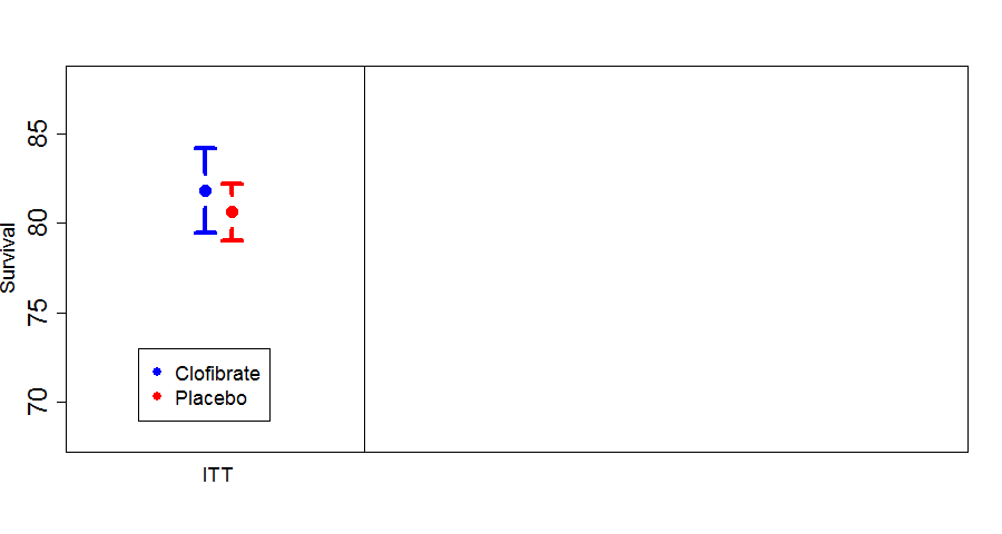
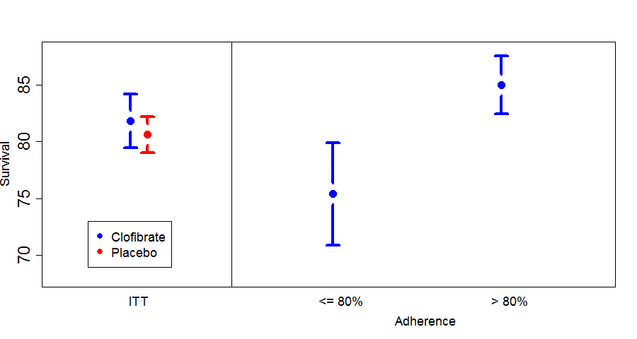
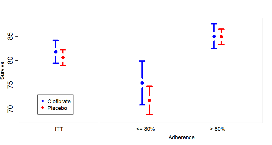
CDP Analysis
ITT analysis showed no difference between groups.
Here is a summary of survival in the clofibrate group by adherence to treatment.
There is a large, highly statistically significant difference in mortality between people taking at least 80% of their assigned medication and those taking less than 80%.
This might suggest that if you take your medication, you will receive a mortality benefit, relative to those who only take part of their medication.
Here we see a difference at least as large between those taking at least 80% of their placebo and those taking less than 80%.
- placebo is highly effective at improving survival, or
- subjects adhering to placebo have better prognoses than those who fail to adhere.
Of course, it’s most likely that subjects discontinue their placebo because they’re doing poorly. That is, subjects who adhere are different than subjects who don’t.
It is likely that the difference within the clofibrate group is driven by a similar phenomenon and is unrelated to any benefit of treatment.
We can see how this works in our hypothetical COPD trial.
Deviations from ITT
Strict ITT Principle
A catchy phrase commonly used to refer to the ITT principal is “analyze as you randomize”. This means:
- A subject is later found to be ineligible — analyze him/her anyway
- A subject doesn’t receive treatment — analyze anyway
- A subject receives wrong treatment — analyze in assigned (not received) group
Let’s discuss each of these cases and whether we can ever deviate from the rules …
Case #1: Found to Be Ineligible
Might not even be part of the correct study population. For example, a study in females, but somehow you enrolled a male. (Big mistake!)
Another possibility: if exclusion is based on safety, the study drug may now be unsafe.
- Certainly, discontinue the drug if time still allows.
- But remove from the analysis?
Eligibility and Causation
While it may seem logical to exclude such subjects from the analysis, we could invalidate our causal interpretation.
If the discovery or assessment of ineligibility could possibly be associated with treatment assignment, all causal bets are off.
However, we can adhere to the spirit of ITT by reviewing every subject for a particular set of eligibility criteria in a systematic way:
- This should be pre-specified, including (a) which criteria and (b) the review process
- This must be done in a blinded way (which is often harder than it sounds)
Case #2: Didn’t Receive Any Treatment
We talked about the perils of not including those receiving partial treatment.
The argument can be extended to not receiving any treatment (after all, no treatment is basically the same as only receiving a very small dose).
However, we may be able to exclude patients not receiving any drug or treatment, without sacrificing a causal interpretation.
Modified ITT (MITT)
This term has been applied to a number of situations in which the analysis did not strictly follow ITT.
In many cases, it has been used in an attempt to make blatant, serious violations of ITT acceptable.
We believe that this misuse has given MITT a bum rap.
A proper definition of MITT is:
An MITT analysis includes every subject who received at least one dose of study drug, or who at least “started” treatment.
Consider a subject in a double-blind trial who is assigned to A but does not receive any treatment. If the blind is very secure then had that same subject been assigned to B, she also would not have received any treatment.
In either case, she would not have received treatment, so in either case, she would have had the same outcome (i.e., whatever outcome would result from receiving no treatment).
In a sense, initiating treatment becomes part of the randomization process (or even the eligibility process), and you can think of the time of first treatment as the randomization time.
If this were a trial of perfect twins, either both twins would initiate treatment, or both twins would never start treatment.
The MITT analysis excludes twins who never start treatment, leaving only complete pairs who took at least one dose, a valid causal analysis.
Case #3: Randomization Errors
(Note: we are not talking about errors in the randomization list itself.)
Imagine the following common scenario:
- A research coordinator is enrolling a patient and is ready to randomize.
- The phone system or website gives a randomization number of “0001”.
- The coordinator writes down “0011” and then proceeds to grab the wrong vial/packet.
- There are other types of events that can lead to a similar situation.
Hope
You might hope that 0001 and 0011 are the same treatment arm.
In that case, you could reset the randomization system to give “0001” when “0011” comes up.
Some problems with this approach:
- This might not be possible, or at least quite difficult.
- This could partially unblind the person enrolling.
- And what if 0001 is Arm A and 0011 is Arm B? If we switch, we have achieved two randomization errors for the price of one.
Different Treatment Arms / Wrong Treatment
What do we do in the analysis?
If we keep the randomization that was supposed to occur, we still achieve a valid causal interpretation. (This is somewhat like considering it a non-adherence problem.)
If we make the assumption that the mistake was “completely random”, or at least independent of the actual treatment assignment, then switching the group to what they actually received gives a valid analysis.
In many cases, this assumption is almost certainly true. However, it is still an additional assumption.
Also, if these errors are rare, there will be little impact on the analysis.
If the errors are common, you have conducted your trial poorly and will have difficulty convincing the skeptic, regardless of how you analyze.
Recommendation: safest route is to analyze based on the treatment that was assigned by randomization. Replace the “kit” that was mistakenly used so it will be there when that randomization number comes up.
The best approach is to prevent the errors in the first place.
If they do occur, always make note of the errors so the skeptic has all the info he/she wants.
A Lot of Wrong Treatments
Occasionally, the following situation, or something similar, could occur:
During routine tests of the study drug, you discover that an entire batch is of bad quality. Many subjects received drug determined to be less effective, or even ineffective.
Do NOT just throw out those subjects in the intervention arm.
You have two options:
- Leave everybody in the analysis.
- Throw out all subjects who could have been randomized to the bad batch of study drug.
The second option is OK, as long as blinding (especially of results) is secure.
Another Type of Error
Suppose randomization is stratified by some characteristic. Information regarding that characteristic is entered into the randomization system. What are the consequences when the wrong information is entered, possibly resulting in the subject being assigned to the “wrong” treatment?
Reminder: Why Stratify?
Stratification in the analysis:
- Improves trial power (possibly)
But why stratify randomization?
- To increase the perception of validity
- To increase power
However, we have already discussed how covariate balance is neither necessary nor sufficient for valid causal inference. So, this reason for stratified randomization is scientifically irrelevant.
In most trial designs, the increase in power would be so small, it’s negligible. Certainly, an imbalance of a few patients would have a negligible effect on power.
Conclusion: there are no compelling reasons to stratify randomization and nothing that could affect the causal bridge.
Wrong Stratum
The subject still received a valid randomization — the causal properties of randomization still hold.
The analysis (if stratified) should use the correct stratum information and the treatment group that was actually assigned by the randomization.
Summary
Randomization
The purpose of randomization is NOT:
- to “estimate the treatment effect”
- to balance the baseline covariates
Neither of these is required for for valid causal inference.
The purpose of a randomized trial is to establish a causal relationship between an intervention and outcome.
In order to determine whether a treatment has a causal effect on an outcome, we must either:
- Be omniscient
- Have a population of perfect twins
- Randomize
Randomization is the only one of these that we can do in the real world.
Missing Data
Missing data compromise the causal interpretation of the analysis of a trial.
Analytical methods for dealing with missing data (including complete-case analysis) do not adequately restore the pure causal relationship.
Non-adherence and ITT
Randomization and intention-to-treat analysis are tied together, and both are required for valid causal inference.
The only question that can be answered in a valid way is the question of treatment assignment.
No analysis can give a valid answer to the question
“If you take your medicine, does it work?”unless you force subjects to adhere to their assigned treatment or make unverifiable assumptions.
Importance of Post-Treatment Follow-Up
- It would be nice to estimate the full-adherence effect.
- We can’t do this ethically in human trials, and the “full-adherence” effect might not even be well definied. The “per-protocol” analysis does not help.
- The only causal conclusions we can draw relate to the effect of assignment to treatment.
- To draw these conclusions, we must not (deliberately!) introduce missing data by excluding non-adherers.
- If, by design, our data collection ends when treatment ends (e.g., stop routine visits, stop laboratory tests, track adverse events for only 30 days following discontinuation), we intentionally make key data unavailable for determining the causal effect of assignment to treatment.
- This design decision will sabotage our trial!
If our trial results are to be interpretable, we must understand:
| WITHDRAWAL FROM TREATMENT | ≠ | WITHDRAWAL FROM STUDY |
There must be a process in place for withdrawing from treatment without withdrawing from data collection.
Withdrawal from data collection should be extremely rare.
We must follow and collect data on all subjects, regardless of adherence to treatment.
Key Points
The purpose of a randomized trial is to establish a causal relationship between an intervention and outcome.
ITT is the only analytical approach that relies solely on randomization to infer the effectiveness of treatment.
| WITHDRAWAL FROM TREATMENT | ≠ | WITHDRAWAL FROM STUDY |
Backup Slides
Non-inferiority Trials
Purpose of Non-Inferiority Trials
Non-inferiority trials are intended to show that an experimental treatment is no worse than a control treatment.Conventional Wisdom
Convention wisdom says:
Trial conduct that makes the two groups look more similar than they really are will make a finding of non-inferiority more likely, even when the experimental group is actually inferior to control.
We can’t disagree with this comment, but it can be difficult to assess when trial conduct will make groups look more similar.
Trial Conduct Myths
Two myths:
- Non-adherence to assigned treatment makes groups look more similar.
- “Per-protocol” or “As-treated” analysis provide more reliable estimates of the true treatment effect.
Myth #1: Non-adherence Makes Groups More Similar
Myth #1 is typically supported by the following logic:
- If everyone in both group adhered to their assigned treatment, we would reliably estimate the “true” treatment effect.
- If no one in either group adhered to their assigned treatment, the two groups would be identical and we would find (up to statistical uncertainty) that there is no difference between groups.
- Therefore, if we have partial adherence, the estimated treatment effect would be somwhere between the “true” treatment effect and no treatment effect.
Obvious, right?
Unfortunately, while #1 and #2 are plausible, there is no reason to believe #3.


Debunking Myth #1
Suppose that:
- larger responses correspond to better outcomes
- the experimental treatment is more effective than the control
- and both are more effective than the “rescue treatment” that subjects receive if they discontinue from their assigned treatment.
Myth #2: Per-Protocol Analysis is More Reliable
Finally, regarding Myth #2, we have already seen that “Per-protocol” or “As-treated” analysis do not have a valid causal interpretation, and cannot be relied upon to fix the problem.
The only reliable solution is to perform the best trial possible, perform an ITT analysis, and apply sound scientific judgment.
A Real Example
PolyHeme is a blood substitute. In a non-inferiority trial, subjects with acute blood loss from trauma were randomized to
- polyheme/blood or
- crystaloid/blood
The primary outcome was all-cause mortality with a 7% non-inferiority margin.
The final manuscript presented several analyses. The “as randomized” analysis (top) excluded 6 untreated subjects, though it gave similar results to an ITT analysis.
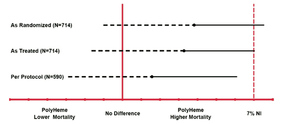
Here are the results in tabular form:
| ITT | Per-Protocol | Violators | |||||||
|---|---|---|---|---|---|---|---|---|---|
| N | Dead | % | N | Dead | % | N | Dead | % | |
| Polyheme | 355 | 48 | 13.5 | 279 | 31 | 11.1 | 71 | 16 | 22.5 |
| Control | 365 | 36 | 9.9 | 311 | 29 | 9.3 | 53 | 6 | 11.3 |
The p-value for PP versus Violators within the Polyheme group is 0.012. The “violators” in the Polyheme group were likely higher risk subjects than the adherers.
No other comparisons reach “statistical significance.”
Remember …
- The premise for using PP is that violators look more like controls, shrinking the ITT difference.
- There is no evidence of that here!